How is “healthy” decided when interpreting tumor marker tests?
The National Cancer Institute defines a tumor marker as “a substance found in tissue, blood, or other body fluids that may be a sign of cancer or certain benign (noncancerous) conditions.” This statement provides both the major advantage and the major disadvantage of such substances: they are made by both normal and cancerous cells and can be found in elevated amounts in benign and malignant conditions. Currently, no tumor marker is accepted as being so specific that it points to only one type of cancer. This reality can be demonstrated with an initial exploration of the most critical terms associated with such medical decisions: diagnostic sensitivity, diagnostic specificity, positive predictive value, and negative predictive value.
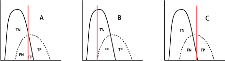
When used in a selected population, the majority of tumor marker tests (and even most diagnostic tests!) will demonstrate a bimodal pattern, with one curve showing the test results for “healthy” individuals and the other curve showing those with the disease in question. It is common for those two curves to intersect (Figure A). The crucial aspect here is the placement of the cutoff value, which will distinguish the true-positives (TP, persons with the disease) from the true-negatives (TN, without the disease) clinically. Inevitably, however, the placement of the cutoff value will result in some healthy individuals being called “positive” (false positive, FP) and some with the disease being called “negative” (false negative, FN). Moving that cutoff point to the left (Figure B) to maximize the number of true-positive results identified by the test automatically increases the number of false-positives; accordingly, moving the cutoff to the right (Figure C) will increase the number of false-negatives.
The clinical decision for where that line should be placed can depend on the severity of the cancer and the availability of treatment and is usually the result of a consensus of medical personnel who are experts in each kind of cancer.
)
What does “moving the line” do in establishing predictive values of tumor marker tests?
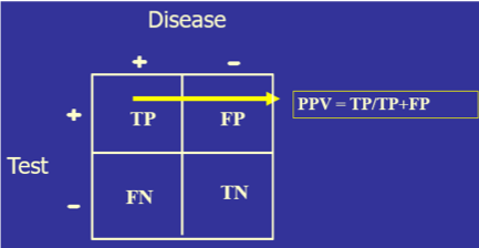
Ideally, the closer that a laboratory test can get to correctly identifying all those with disease as positive and all those without disease as negative, the more diagnostically useful that test will be. This can be determined mathematically by setting a test cutoff at a certain level, counting the number of the tested population who fit into TP, FP, TN, and FN, and then placing those values in a 2x2 table.
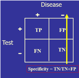
The test’s diagnostic sensitivity is the percentage of those with the disease who have a positive test. Conversely, the test’s diagnostic specificity is the percentage of those without the disease who have a negative test.
Four things to notice:
- The higher the calculated percentage, the better the test is for detecting TP or TN.
- The numbers in each cell of the 2x2 table depend on where the line is! When the line changes, the numbers in each cell change, which changes the sensitivity and specificity.
- Both sensitivity and specificity imply that you already know if the person has the disease or not. Diagnoses, of course, do not work that way since the clinician may have a hypothesis about the patient’s condition, but use the clinical laboratory tests to confirm or disprove that hypothesis. For this reason, another set of calculations is needed: positive predictive value (PPV, the percentage of those with a positive test who have the disease) and negative predictive value (NPV, the percentage of those with a negative result who do not have the disease). So, sensitivity/specificity looks at the data from the disease standpoint, and PPV/NPV look at the same data from the test standpoint.
- These terms are not the same as analytical sensitivity/specificity, which, respectively, describe the smallest concentration the method can distinguish from “zero” and the ability of the method to measure what you want it to measure.
)
Diagnostic sensitivity and specificity are the criteria used for choosing whether to offer a screening test (“By using this test, how much am I willing to risk missing someone who actually has the disease?”), while PPV/NPV become the diagnostic tools when obtaining the test result before knowing the final diagnosis and then asking, “How reliably will this result predict that this patient truly has or truly does not have the condition?”
How is clinical lab testing like a World War II radar operator?
The statistics above can also be visualized in a tool that was originally used in World War II to establish the ability of radar operators in distinguishing between enemy aircraft (TP) and noise (FP). These “receiver operating characteristic” (ROC) plots were introduced into medical decision making as early as the 1950s and soon were found useful in many areas, including psychology, medical imaging, and diagnostic lab testing. These curves display the data obtained when multiple sequential cutoff test values, as illustrated below, determine the proportion of the tested population who will be TP and FP.
By “moving the line,” redoing the numbers in the 2x2 table, recalculating the sensitivity (TP) and specificity (TN), and finally subtracting the specificity (TN%) from 1 to get the FP%, you now have an x,y point at that cutoff value. Moving the line repeatedly and repeating the calculations at each move eventually gives a set of points to place on the ROC curve:
Each x,y point on the curve represents the same testing population with only the cutoff line being moved. The most useful test, especially for a tumor marker, is one which gives the highest rate of true positives (1.0 on the y-axis) and the smallest rate of false positives (0 on the x-axis). Therefore, the most useful test is one whose ROC curve moves closest to the upper left corner of the ROC graph (yellow in the figure). The least useful will be one which is closest to the mid-diagonal line (blue in the figure).
As an example, two tumor marker tests, CA125 and HE4, were compared in a patient population known to have ovarian cancer, with the resulting ROC curves displayed here.
Note that the curve for HE4 (red) is closer to the upper left corner, so it would be the better discriminator for ovarian cancer.
Note also that an additional calculation is provided in the table: AUC (area under the curve). The higher the AUC is to 1.00, the better the test. Here, again, with an AUC of 0.96, the HE4 test is better than the CA125 test.
Why can’t we screen whole populations for cancer using tumor markers?
Despite how often we hear about cancer occurring today, it actually is a rare phenomenon, especially when looking at total populations. The reality is similar to doing flu testing. Since that is a seasonal disease, testing for it is only done in those months where the possibility of having a higher TP percentage is possible. Otherwise, it would be a waste of resources since the numbers of TP could be very low. This is the concept of prevalence: the proportion of a population who at this moment in time has a condition. Prevalence differs from incidence rate, the number of new cases per population at risk in a given time period.
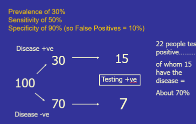
Let’s look at a disease whose prevalence is 30% and a diagnostic test whose sensitivity is 50% and specificity is 90%. Take 100 individuals from a population and use the test on their samples. The prevalence says that out of those 100 people, 30 of them will have the disease and 70 will not. The 50% sensitivity says that 15 of the 30 will give a positive test result (TP). Specificity at 90% says that 63 will have a negative result (TN), and 7 will have a positive result (FP). The total number of “positives” is 15 plus 7 = 22, of which 15 truly have the disease, so the PPV is about 70%.
)
Let’s now change the prevalence of the disease to 4% and use the same diagnostic test as before (sensitivity 50%, specificity 90%). Take 100 individuals from that population and use the test on their samples. The 4% prevalence says that out of those 100 people, only 4 of them will have the disease and 96 will not. The sensitivity says that 2 of the 4 with disease will give a positive test result (TP). Specificity says that 86.4 patients will have a negative result (TN), and 9.6 will have a positive result (FP). The total number of “positives” is 2 plus 9.6 = 11.6, of which 2 truly have the disease, so the PPV is about 17%.
Since the prevalence of cancer in the general population is so rare, the PPV would be very low if a tumor marker test were done as a general screening test. The PPV increases, sometimes significantly, when the testing is done on targeted populations: those with familial cancer backgrounds, those with symptoms, etc., since the prevalence % increases in that population.
What are useful tumor marker classifications and examples?
Tumor markers fall into five categories:
- Oncofetal antigens
- Hormones
- Carbohydrates
- Enzymes
- DNA/RNA
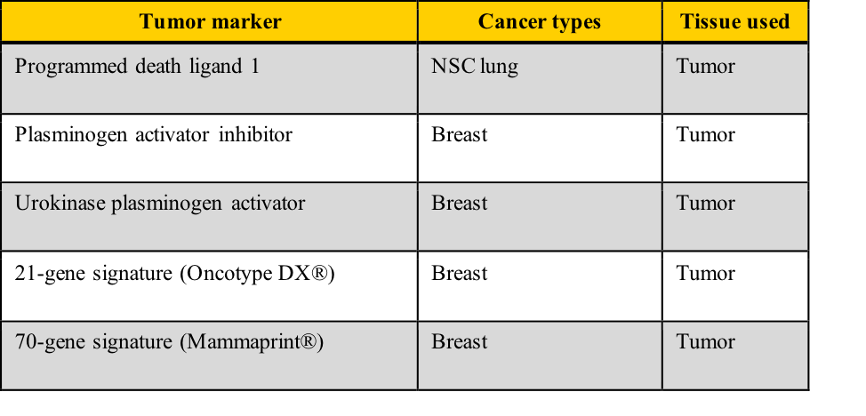
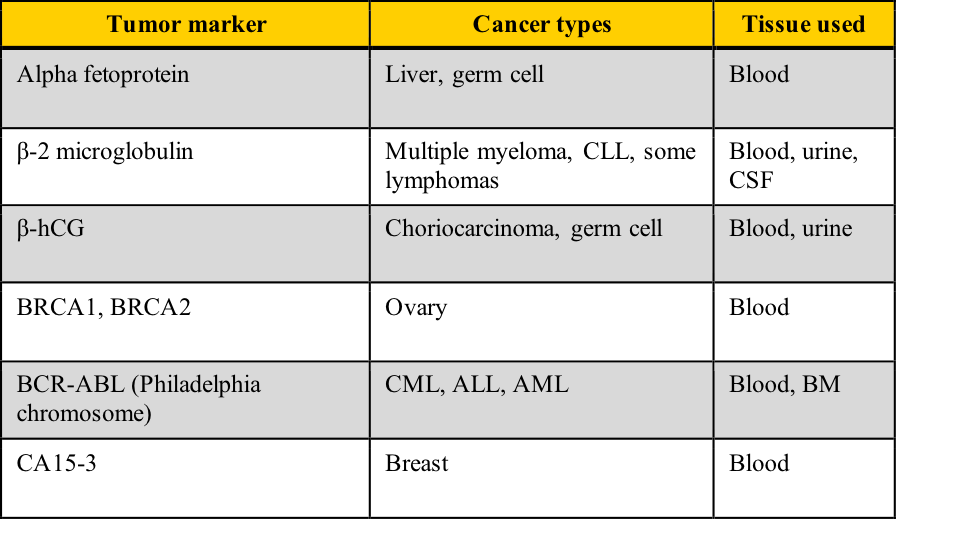
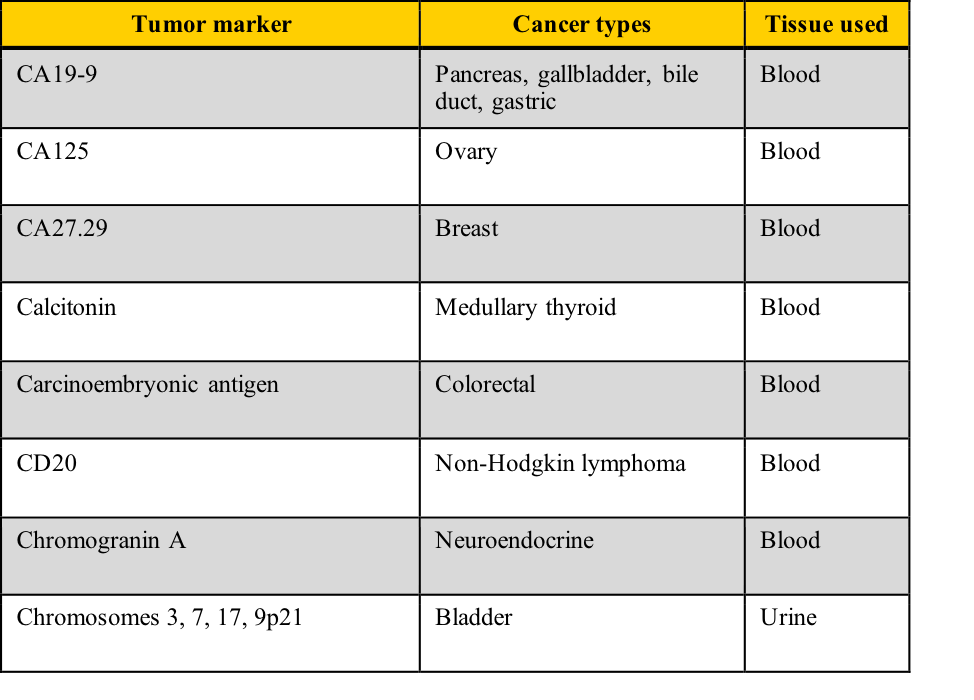
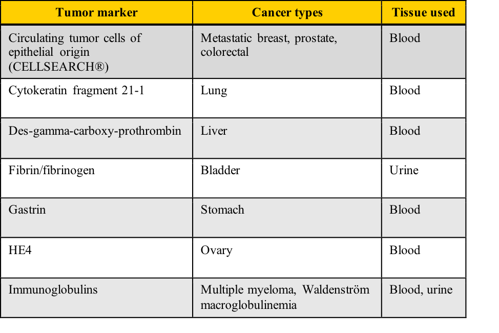
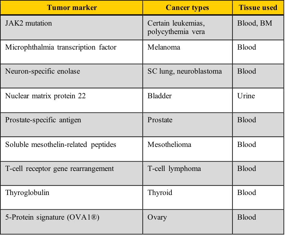
Examples of tumor markers, their most common tumor associations, and the tissue used for the testing include those listed in this table. Note the cancer types which have more than one tumor marker and those for which few tumor markers are available.
 A cancer diagnosis is one of the most frightening situations in healthcare. It conjures up multiple diagnostic tests, painful therapy, an uncertain future, and the dreaded “wait-and-see.” Your challenge in this module includes determining how “healthy” is decided with tumor marker lab tests, calculating diagnostic sensitivity/specificity and positive/negative predictive values, and correlating those calculations with ROC curve predictions.
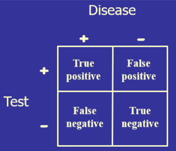) The test’s diagnostic sensitivity is the percentage of those with the disease who have a positive test. Conversely, the test’s diagnostic specificity is the percentage of those without the disease who have a negative test.
The test’s diagnostic sensitivity is the percentage of those with the disease who have a positive test. Conversely, the test’s diagnostic specificity is the percentage of those without the disease who have a negative test.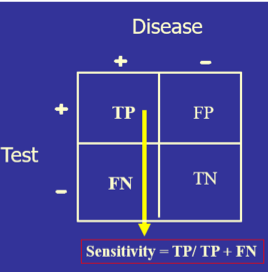)
) Four things to notice:
Four things to notice: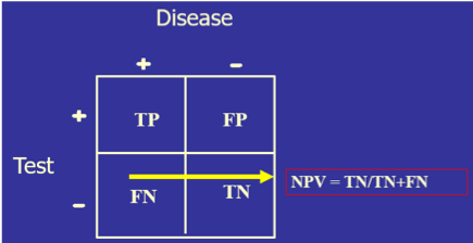) Diagnostic sensitivity and specificity are the criteria used for choosing whether to offer a screening test (“By using this test, how much am I willing to risk missing someone who actually has the disease?”), while PPV/NPV become the diagnostic tools when obtaining the test result before knowing the final diagnosis and then asking, “How reliably will this result predict that this patient truly has or truly does not have the condition?”
Diagnostic sensitivity and specificity are the criteria used for choosing whether to offer a screening test (“By using this test, how much am I willing to risk missing someone who actually has the disease?”), while PPV/NPV become the diagnostic tools when obtaining the test result before knowing the final diagnosis and then asking, “How reliably will this result predict that this patient truly has or truly does not have the condition?”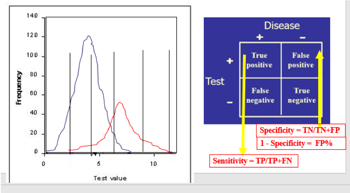) By “moving the line,” redoing the numbers in the 2x2 table, recalculating the sensitivity (TP) and specificity (TN), and finally subtracting the specificity (TN%) from 1 to get the FP%, you now have an x,y point at that cutoff value. Moving the line repeatedly and repeating the calculations at each move eventually gives a set of points to place on the ROC curve:
By “moving the line,” redoing the numbers in the 2x2 table, recalculating the sensitivity (TP) and specificity (TN), and finally subtracting the specificity (TN%) from 1 to get the FP%, you now have an x,y point at that cutoff value. Moving the line repeatedly and repeating the calculations at each move eventually gives a set of points to place on the ROC curve: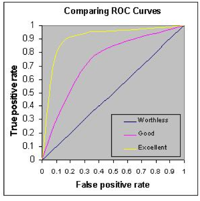) Each x,y point on the curve represents the same testing population with only the cutoff line being moved. The most useful test, especially for a tumor marker, is one which gives the highest rate of true positives (1.0 on the y-axis) and the smallest rate of false positives (0 on the x-axis). Therefore, the most useful test is one whose ROC curve moves closest to the upper left corner of the ROC graph (yellow in the figure). The least useful will be one which is closest to the mid-diagonal line (blue in the figure). As an example, two tumor marker tests, CA125 and HE4, were compared in a patient population known to have ovarian cancer, with the resulting ROC curves displayed here.
Each x,y point on the curve represents the same testing population with only the cutoff line being moved. The most useful test, especially for a tumor marker, is one which gives the highest rate of true positives (1.0 on the y-axis) and the smallest rate of false positives (0 on the x-axis). Therefore, the most useful test is one whose ROC curve moves closest to the upper left corner of the ROC graph (yellow in the figure). The least useful will be one which is closest to the mid-diagonal line (blue in the figure). As an example, two tumor marker tests, CA125 and HE4, were compared in a patient population known to have ovarian cancer, with the resulting ROC curves displayed here.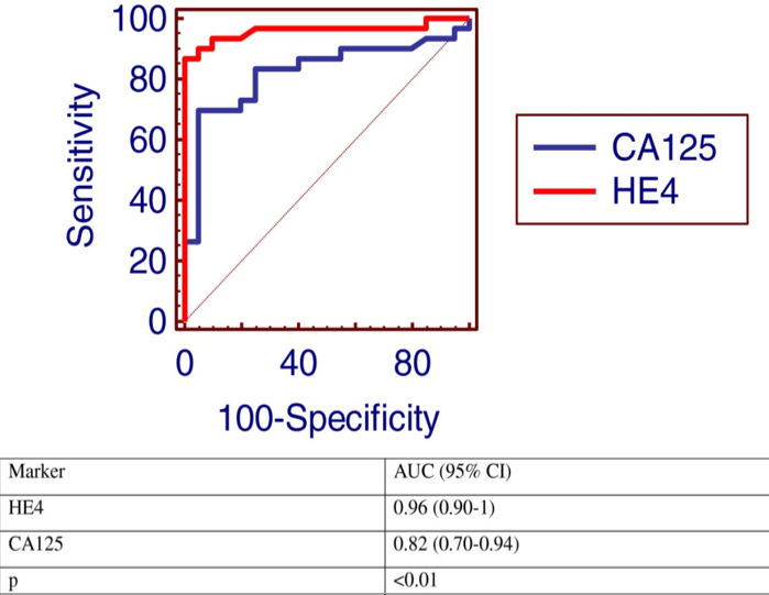) Note that the curve for HE4 (red) is closer to the upper left corner, so it would be the better discriminator for ovarian cancer. Note also that an additional calculation is provided in the table: AUC (area under the curve). The higher the AUC is to 1.00, the better the test. Here, again, with an AUC of 0.96, the HE4 test is better than the CA125 test.
Note that the curve for HE4 (red) is closer to the upper left corner, so it would be the better discriminator for ovarian cancer. Note also that an additional calculation is provided in the table: AUC (area under the curve). The higher the AUC is to 1.00, the better the test. Here, again, with an AUC of 0.96, the HE4 test is better than the CA125 test.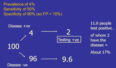) Since the prevalence of cancer in the general population is so rare, the PPV would be very low if a tumor marker test were done as a general screening test. The PPV increases, sometimes significantly, when the testing is done on targeted populations: those with familial cancer backgrounds, those with symptoms, etc., since the prevalence % increases in that population.
Since the prevalence of cancer in the general population is so rare, the PPV would be very low if a tumor marker test were done as a general screening test. The PPV increases, sometimes significantly, when the testing is done on targeted populations: those with familial cancer backgrounds, those with symptoms, etc., since the prevalence % increases in that population.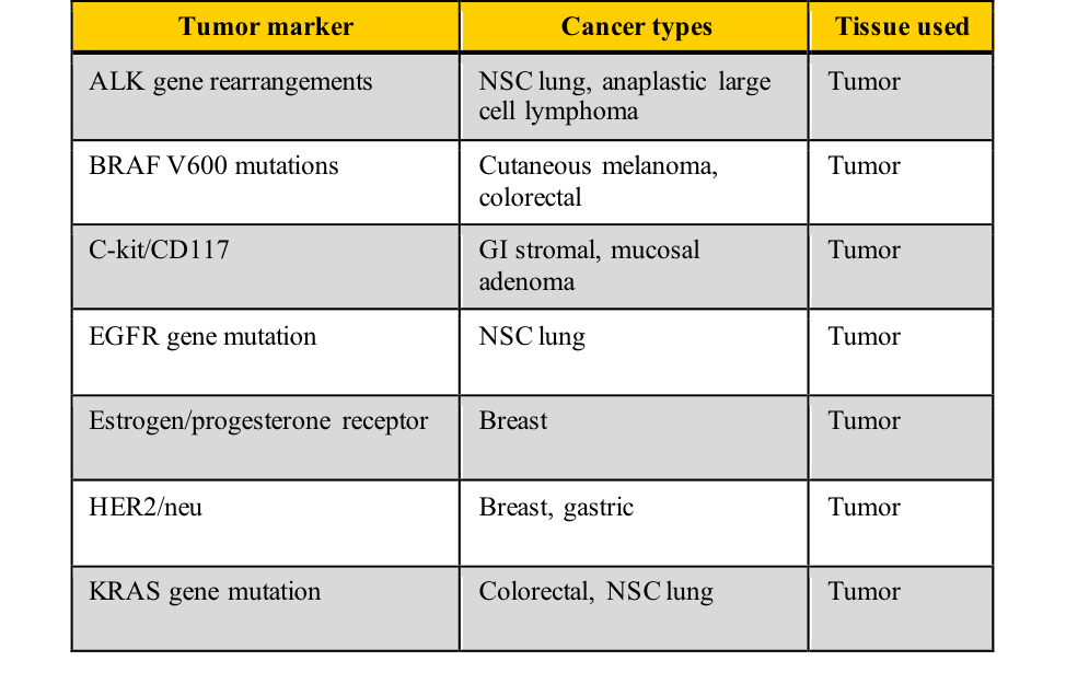)
)
)
)
)
)